A close look at matrices

1. Introduction.

There is a tendency among mathematicians to regard matrices as arcane and mystic entities, with cryptic properties which reward a lifetime of study. Engineers can be duped into this point of view if they are not careful.

Matrices are, in fact, just a form of shorthand that can come in very useful when a lot of calculating operations are involved. There are strict rules to observe, but when used properly they are mere tools which are the servant of the engineer.

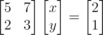
You will probably have first encountered matrices in the solution of simultaneous equations.

To take a simple example, the equations:

5 x + 7 y = 2

and

2 x + 3 y = 1

can be "tidied up" by separating the coefficients from the variables in the form:

$\begin{bmatrix} 5& 7\\ 2& 3\end{bmatrix}\begin{bmatrix}x\\y\end{bmatrix}=\begin{bmatrix}2\\1\end{bmatrix}$

where the variables are now conveniently grouped as a vector.

Now this 'close relationship' with simultaneous equations forces a convention on us that will haunt us in almost every application! For a start, we are generally committed to representing our vectors as 'columns', one number above the other. We can easily include in our technical paper the expression

A z = b

but when we want to list the value of z we must either take up a couple of text lines with coefficients one above the other, or else give the value of its 'transpose' and write (x, y)^T or (x, y)'

Now the multiplication rule has defined itself.

We move across the top row of the matrix, multiplying each element by the corresponding component as we move down the vector, adding up these products as we go. The total is the top element of the vector result, here 5 x + 7 y.

Then we do the same for the next row, and so on.

2. More on vectors

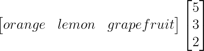
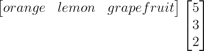
So what does a vector actually 'mean'? The answer has to be, "anything you like". Anything, that is, that cannot be represented by a single number but requires a string of numbers to define it. It could even be a shopping list.

5 oranges + 3 lemons + 2 grapefruit

can be written as

$\begin{bmatrix} orange&lemon&grapefruit\end{bmatrix}\begin{bmatrix}5\\3\\2\end{bmatrix}$

(orange, lemon, grapefruit) (5, 3, 2)'

where the 'dash' denotes a transpose, or else put the dot between them that we use for 'scalar product'. The numbers on the right have defined a 'mixture' of the items on the left.

Rather than fruit, we are more likely to apply vectors to coordinate systems - but we are still just picking from a list.

We might define i, j and k to be 'unit vectors' all at right angles, say East, North and Up. We can call them 'basis vectors'.

When we say that point P has coordinates (2, 3, 4)' we mean that to get there you start at the origin and go two metres East, then three metres North and 4 metres Up.

We could write this as

2 i + 3 j + 4 k

a mixture of the basis vectors defined by a matrix multiplication - vectors are just skinny matrices.

Now when we turn our minds to applications, we can see many uses for vector operations. When a force F moves a load a distance x, the work done is given by their scalar product F . x

As before we take products of corresponding elements and add them up, to get a scalar number.

We usually think in terms of "the matrix multiplies the vector". But how about thinking of the vector multiplying the matrix? What does it do to it?

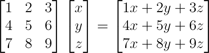
$\begin{bmatrix}1&2&3\\4&5&6\\7&8&9\end{bmatrix}\begin{bmatrix}x\\y\\z\end{bmatrix}=\begin{bmatrix}1x+2y+3z\\4x+5y+6z\\7x+8y+9z\end{bmatrix}$

Well from one point of view, the top element of the answer on the right is equal to the scalar product of the top row of the matrix with the vector (x, y, z)'.
Similarly the other elements are the scalar products of the vector with the middle and bottom rows of the matrix, respectively.

So we have

The product of a matrix and a (column) vector is made up
of the scalar products of the vector with each of the rows of the matrix

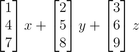
But there is another way of seeing it. The answer is the same as:

$\begin{bmatrix}1\\4\\7\end{bmatrix}x+\begin{bmatrix}2\\5\\8\end{bmatrix}y+\begin{bmatrix}3\\6\\9\end{bmatrix}z$

The product of a matrix and a column vector is a mixture of the vectors that make up the columns of the matrix

So if instead of describing P by the sum of components i, j and k of our basis vectors, we based its coordinates (x, y, z)' on three other vectors u, v and w, then we could 'transform the coordinates' by multiplying (x, y, z)' by a matrix made up of columns representing vectors u, v and w to end up with a vector for P as a mixture of i, j and k.

3. Matrix multiplication.

Often we will find a need to multiply one matrix by another. To see this in action, let us look at another simple 'mixing' example.

In a sweetshop, "Sucks", "Munches" and "Chews" are on sale.

Also on sale are "Jumbo" bags each continuing 2 Sucks, 3 munches and 4 Chews,
and "Giant" bags containing 5 Sucks, 6 Munches and only one Chew.

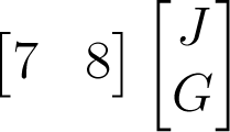
If I purchase 7 Jumbo bags and 8 Giant bags, how many of each sweet have I bought ?

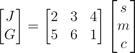
The bag contents can be expressed algebraically as:

J = 2 s + 3 m + 4 c

and

G = 5 s + 6 m + 1 c

or in matrix form as:

$\begin{bmatrix}J\\G\end{bmatrix}=\begin{bmatrix}2&3&4\\5&6&1\end{bmatrix}\begin{bmatrix}s\\m\\c\end{bmatrix}$

Note that matrices do not have to be square, as long as the terms to be multiplied correspond in number.

Now my purchase of 7 Jumbo bags and 8 Giant bags can be written as:

7 J + 8 G

or in grander form as the product of a row vector with a column vector:

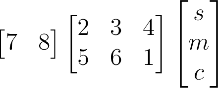
$\begin{bmatrix}7&8\end{bmatrix}\begin{bmatrix}J\\G\end{bmatrix}$

But I can substitute for the J, G vector to obtain:

$\begin{bmatrix}7&8\end{bmatrix}\begin{bmatrix}2&3&4\\5&6&1\end{bmatrix}\begin{bmatrix}s\\m\\c\end{bmatrix}$

To get numerical counts of sucks, munches and chews we have to calculate the product of a numerical row vector with a numerical
matrix. As before, we march across the row(s) of the one on the left, taking the scalar product with the columns on the right.

The answer is what common sense would give.

From 7 Jumbo bags, with Sucks at 2 to a bag, we find 7 times 2 sucks.
From 8 Giant bags we find 8 times 5 more, giving a grand total of 54.

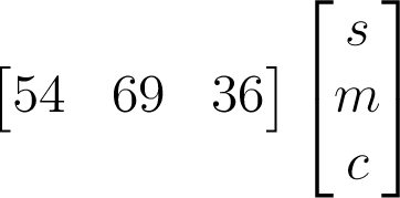
The final answer is

$\begin{bmatrix}54&69&36\end{bmatrix}\begin{bmatrix}s\\m\\c\end{bmatrix}$

i.e. 54 Sucks, 69 munches and 36 chews.

Now the shop is selling an Easter bundle of 3 Jumbo bags and a Giant bag,
and still has in stock Christmas bundles of 2 Jumbo bags and 4 Giant bags.

In no time we can write:

$\begin{bmatrix}E\\C\end{bmatrix}=\begin{bmatrix}3&1\\2&4\end{bmatrix}\begin{bmatrix}J\\G\end{bmatrix}$

In effect, it is a sort of transformation.


Exercise: If I buy 5 Easter packs and one Christmas pack, how many sucks, munches and chews will I have?

Write down the matrices involved and multiply them out by the rules we have found.

(Your answer should be   79 sucks + 105 munches + 77 chews)

The mathematician will still worry about the order in which the matrix multiplication is carried out.
We must not alter the order of the matrices, but we can group the pairs for calculation in two ways.

The Christmas and Easter bags can first be opened to reveal a total of Jumbo and Giant bags,
then these can be expanded into individual sweets,
or alternatively the total of each sweet for a Christmas bag and for an Easter bag can be worked out first;

the result must be the same. (Check it)

The mathematicians would say that "multiplication of matrices is associative" - i.e.

         A B C = (A B) C = A (B C)

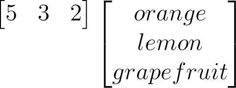
P3.3. Transposition of matrices.

Our mixed fruit multiplication can be written as

$\begin{matrix}\begin{bmatrix}orange&lemon&grapefruit\end{bmatrix}\\\\\\\end{matrix}\begin{bmatrix}5\\3\\2\end{bmatrix}$

or equally well as

$\begin{matrix}\begin{bmatrix}5&3&2\end{bmatrix}\\\\\\\end{matrix}\begin{bmatrix}orange\\lemon\\grapefruit\end{bmatrix}$

giving 5 oranges + 3 lemons + 2 grapefruit in both cases - this result is in the form of a scalar.

But note that in reversing the order in which we multiply the vectors, we have had to transpose them.

Now transposing a scalar is not very spectacular - but when two matrices are multiplied together to give another matrix,

C = A B

then if we wish to find out the transpose of C we must both transpose A and B and reverse the order we multiply them in.

C' = B' A'

So you see that if we had been prepared to write our equations in the form

x' A'

rather than

A x

we could happily have dealt in row vectors instead of column vectors.
Some of the expressions for moving an object around with several transformations would have made more sense, too!

But we are locked in to the conventions as they stand, so enough of grumbling!

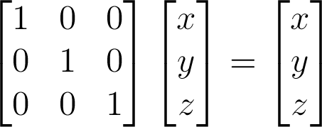
4. The unit matrix

One last point to note before moving on is that:

$\begin{bmatrix}1&0&0\\0&1&0\\0&0&1\end{bmatrix}\begin{bmatrix}x\\y\\z\end{bmatrix}=\begin{bmatrix}x\\y\\z\end{bmatrix}$

The matrix with 1's down its diagonal and 0's elsewhere has the special property that its product with any vector or matrix leaves that vector or matrix unchanged. Of course, there is not just one unit matrix, they come in all sizes to fit the rows of the matrix they have to multiply. This one is the 3 x 3 version.

5. Coordinate transformations.

I mentioned above that vector geometry is usually introduced with the aid of three orthogonal unit vectors i, j and k.

For now, let us keep to two dimensions and consider just (x, y)', meaning x i + y j.

Now suppose that there are two sets of axes in action. With respect to our first set the point is (x, y)'
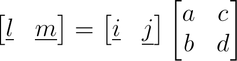
but with respect to a second set it is (u, v)'. Just how can these two vectors be related ?

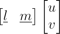
What we have in effect is one pair of unit vectors i and j, and another pair l and m, say.
Since both sets of coordinates represent the same vector, we have:

x i + y j = u l + v m

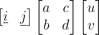
Now each of the vectors l and m must be expressible in terms of i and j.

Suppose that

l = a i + b j

and

m = c i + d j

or in matrix form:

$\begin{bmatrix}\underline{l}&\underline{m}\end{bmatrix}=\begin{bmatrix}\underline{i}&\underline{j}\end{bmatrix}\begin{bmatrix}a&c\\b&d\end{bmatrix}$

We want the relationship in this slightly twisted form, because we want to substitute into

$\begin{bmatrix}\underline{l}&\underline{m}\end{bmatrix}\begin{bmatrix}u\\v\end{bmatrix}$

to eliminate vectors l and m to get:

$\begin{bmatrix}\underline{i}&\underline{j}\end{bmatrix}\begin{bmatrix}a&c\\b&d\end{bmatrix}\begin{bmatrix}u\\v\end{bmatrix}$

Now the ingredients must match, i.e.

$\begin{bmatrix}x\\y\end{bmatrix}=\begin{bmatrix}a&c\\b&d\end{bmatrix}\begin{bmatrix}u\\v\end{bmatrix}$

Although this exercise is now graced with the name "vector geometry", we are merely adding up mixtures in just the same form as the antics in the sweetshop.

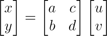
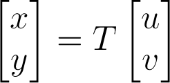
To convert our (u, v)' coordinates into the (x, y)' frame, we simply multiply the coordinates by an appropriate matrix which defines the mixture.

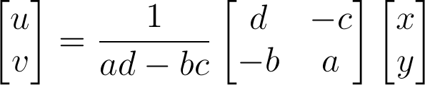
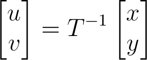
Suppose however we are presented with the values of x and y and are asked
to find (u, v)'. We are left trying to solve two simultaneous equations:

x = a u + c v

and

y = b u + d v

In traditional style we multiply the top equation by d and subtract c times the second equation to obtain:

d x - c y = (ad - bc) u

and in a similar way we find

-b x + a y = (ad - bc) v

which we can rearrange as

$\begin{bmatrix}u\\v\end{bmatrix}=\frac{1}{ad-bc}\begin{bmatrix}d&-c\\-b&a\end{bmatrix}\begin{bmatrix}x\\y\end{bmatrix}$

where the constant 1/(ad - bc) multiplies each of the coefficients inside the matrix.
If the original relationship between (x, y)' and (u, v)' was

$\begin{bmatrix}u\\v\end{bmatrix}=T^{-1}\begin{bmatrix}x\\y\end{bmatrix}$

then we have found an 'inverse matrix' such that

$\begin{bmatrix}u\\v\end{bmatrix}=T^{-1}\begin{bmatrix}x\\y\end{bmatrix}$

The value of (ad - bc) obviously has special importance -
we will have great trouble in finding an inverse if (ad - bc) = 0.
Its value is the 'determinant' of the matrix T.

6. Matrices, notation and computing.

In a computer program, rather than using separate variables x, y, u, v and so on,
it is more convenient mathematically to use "subscripted variables" as the elements of a vector.
The entire vector is then represented by the single symbol x, which will be made up of elements
x₁, x₂ and so on.

Matrices are now made up of elements with two suffices, thus:

A =

a₁₁ a₁₂ a₁₃

a₂₁ a₂₂ a₂₃

a₃₁ a₃₂ a₃₃

In a computer program, the subscripts appear in brackets, so that a vector could be represented by the elements X(1), X(2) and X(3), while the elements of the matrix are A(1,1), A(1,2) and so on.

It is in matrix operations that this notation really earns its keep. Suppose that we have a relationship

x = T u

where the vectors have three elements and the matrix is 3 by 3. Instead of a massive block of arithmetic,
the entire product is expressed in just five lines of Basic program:

FOR
I=1
TO
3

X(I)=0

                    FOR J=1 TO 3 
X(I)=X(I)+T(I,J)*U(J)

                    NEXT J

NEXT I

For the matrix product C = A B the program is hardly any more complex:

FOR I=1
                    TO 3

FOR J=1
                    TO 3

C(I,J)=0

FOR K=1
                    TO 3

C(I,J)=C(I,J)+A(I,K)*B(K,J)

NEXT K

                  

NEXT J

                  

NEXT I 

                  

or in Java or C it becomes:

for( i =
                    1; i<=3; i++){   

                       for( j = 1; j<=3; j++) { 

                          c[i][j] = 0;

                          for (k = 1;
                    k<=3;k++) {

c[i][j]

                    +=  a [i][k]*b[k][j];

                          }

                       }

                    }

These examples would look almost identical in a variety of languages and would show the same economy of programming effort.
In Matlab the shorthand of matrix operations goes even further - but there is a danger that the engineroom will be lost to view behind the paintwork.

Clearly if we are to try to analyse any but the simplest of systems by computer,
we should first represent the problem in a matrix form.

But beware!!

If you have no computer to hand, it will almost certainly be quicker, easier and less prone to errors to use non-matrix methods to solve the problem.